
Deephams STW – CFD Modelling (2016)
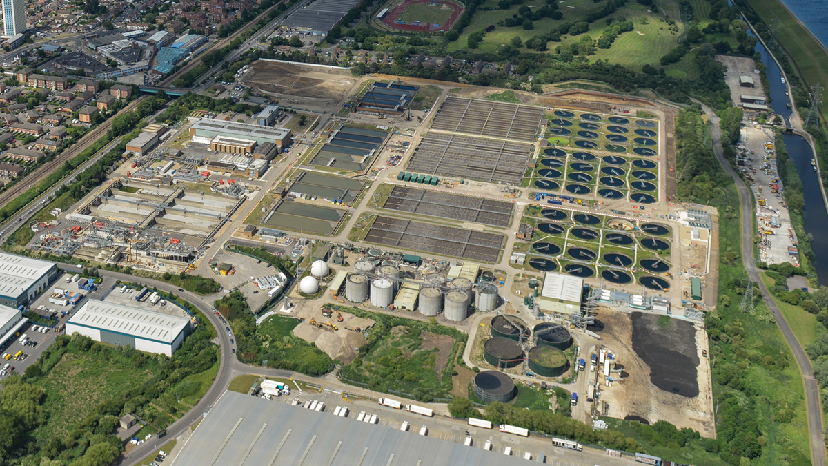
Deephams STW - Courtesy of AMK JV/Thames Water
Deephams STW, which is located in East London, is the ninth largest works in the UK and serves a population equivalent of 891,000 (as of 2011) [1]. In order to cater for increasing population growth, meet new wastewater quality standards, be prepared for weather variations and to replace an ageing plant, a major upgrade has been undertaken by phased replacement of existing treatment streams. The upgrade includes new primary settlement tanks, activated sludge plant (ASP) lanes and final settlement tanks (FSTs), with the capacity of the new treatment streams being greater than the streams being replaced.
[1] Thames Water, A630 Deephams Sewage Treatment Works Upgrade, Project Overview Report, Phase 2 Public Consultation Version, Feb 2014.
Computational fluid dynamics
In order to remove phosphorous, dosing with ferric sulphate takes place in a mixing chamber, from which the flow then passes to flocculation chambers prior to distribution to the primary tanks. Effluent from the primary tanks is distributed to 6 (No.) ASP lanes, which comprise anoxic zones and aeration lanes. Final settlement takes place in 10 (No.) FSTs, each FST being 45m in diameter.
MMI assisted the design team by undertaking computational fluid dynamics (CFD) analysis of the mixing chamber, aeration lanes and FSTs in order to demonstrate that the designs were robust and to provide design solutions where performance was not ideal.
Mixing chamber
Flows received by the flow to full treatment (FTFT) pumping station are pumped to a high energy mixing chamber (HEMC) where ferric sulphate is added at a concentration of 45%w/w. It is required that the ferric sulphate ‘flash’ mixes (i.e. mixes within a very short time period), due to the ferric sulphate, which oxidises rapidly.
A view of the channel configuration is presented in Figure 1 (below). The positions marked ‘Inlets’ approximate the positions at which flow enters from the pumps. The flow then passes in to a channel that deepens downstream of the pumps and which contains a baffle wall across the channel. It is this region that is referred to as the ‘mixing chamber’. Downstream of the baffle, the flow splits with the flow ultimately being passed to the PSTs.
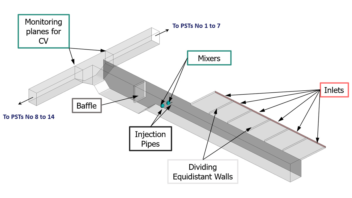
Figure 1: Layout of mixing chamber – Courtesy of MMI Engineering
Based on physical trials, it was required to maintain the baffle as it had been demonstrated that the baffle introduced turbulence and hence mixing.
Three options were assessed in order to optimise the configuration for best mixing. These were:
- Mixing in the absence of mechanical mixers/impellers with ferric sulphate released from a sparge pipe upstream or downstream of the baffle, as shown in Figure 2.
- Impellers located just upstream of the baffle and ferric sulphate injected just downstream of the impeller as shown in Figure 3.
- Impellers located in the channel facing upstream as shown in Figure 1.
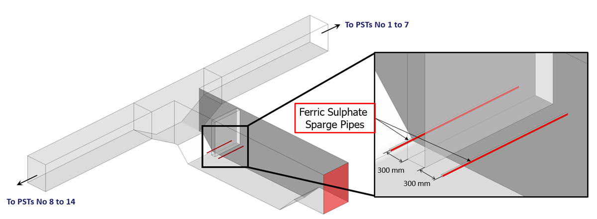
Figure 2: Layout of mixing chamber with ferric sulphate released from sparge pipes – Courtesy of MMI Engineering
The ferric sulphate was solved as an additional fluid with a density of 1,570kg/m3 corresponding to ferric sulphate at 45%w/w. The mixture density, as the ferric sulphate solution was diluted with the waste water stream, was then based on a volume weighted average. A rheology model was also included based on empirical data, so that at high concentration, the ferric sulphate had higher viscosity and hence, a reduced and representative propensity to mix.
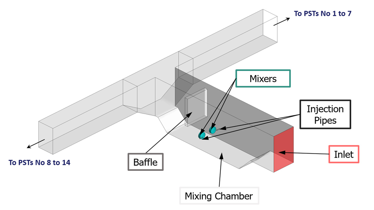
Figure 3: Layout of mixing chamber with mixers in the chamber – Courtesy of MMI Engineering
Assessment of the degree of mixing was quantified by the coefficient of variation (CV): CV=σ/μ, where σ is the standard deviation and μ is the mean value of the variable. The CV for a single variable describes the dispersion of that variable in a non-dimensional form by normalising against the mean. The higher the CV, the greater the dispersion of the variable. The CV was monitored at two locations as presented in Figure 1.
It was found that, in the absence of mixers, the baffle by itself was not able to generate sufficient turbulence to rapidly mix the ferric sulphate and even with mixers, although better, the ferric sulphate did not mix rapidly. With the mixers located upstream in the channel that had reduced depth and hence reduced volume for greater energy input per unit volume in addition to higher energy in the flow, it was found that mixing was much improved. This was observed by both the coefficient of variation and also the concentration of ferric sulphate, which reduces rapidly from the point of injection, as can be seen from the contour plots in Figure 4.
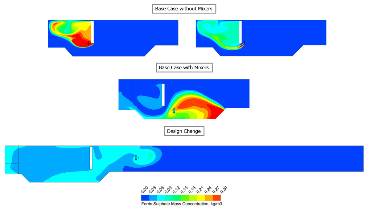
Figure 4: Distribution of ferric sulphate in each assessment – Courtesy of MMI Engineering
Aeration lanes
A view of the arrangement of the anoxic and aeration lanes is presented in Figure 5 (below). Due to the high level weir from the anoxic zones being located in one corner, there was concern as to whether there would be adequate distribution of flow and solids load across the full width of the aeration lane.
Additionally, at maximum flow, there was concern as to whether reverse flow would occur across the weir from the aeration lane in to the anoxic zone. This would not be beneficial to the treatment process as it is undesirable that fluid containing dissolved oxygen (DO) enters a zone that is depleted in DO. In each aerobic zone indicated in Figure 5, aeration grids are used to introduce air.
In order to assess whether reverse flow occurs across the weir, hand/spreadsheet calculations were undertaken to determine the water levels and these were used to verify the levels determined in the CFD calculation.
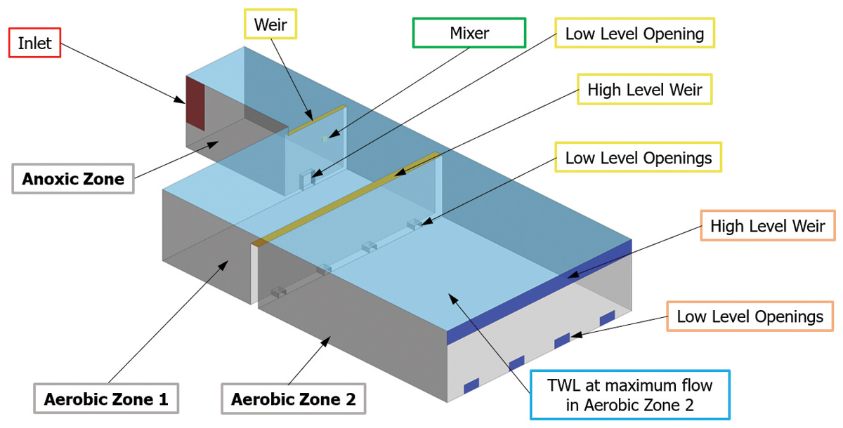
Figure 5: Arrangement of the anoxic and aerobic zones – Courtesy of MMI Engineering
The CFD model was used to assess the flow around the weir and demonstrate whether reverse flow occurred. The calculation considered the increase in density and viscosity of the fluid due to the presence of activated sludge in addition to the bubble induced momentum transfer by resolving the air bubbles in a multiphase calculation.
A view of the velocity vectors at the water surface is presented in Figure 6 showing that reverse flow does not occur.
The flow and load distribution across the low level openings in the aeration lane was assessed over a range of flows and it was found that the distribution of flow was relatively even. It was also found that the activated sludge remained well mixed and hence, the distribution of solids was similar to the flow distribution.
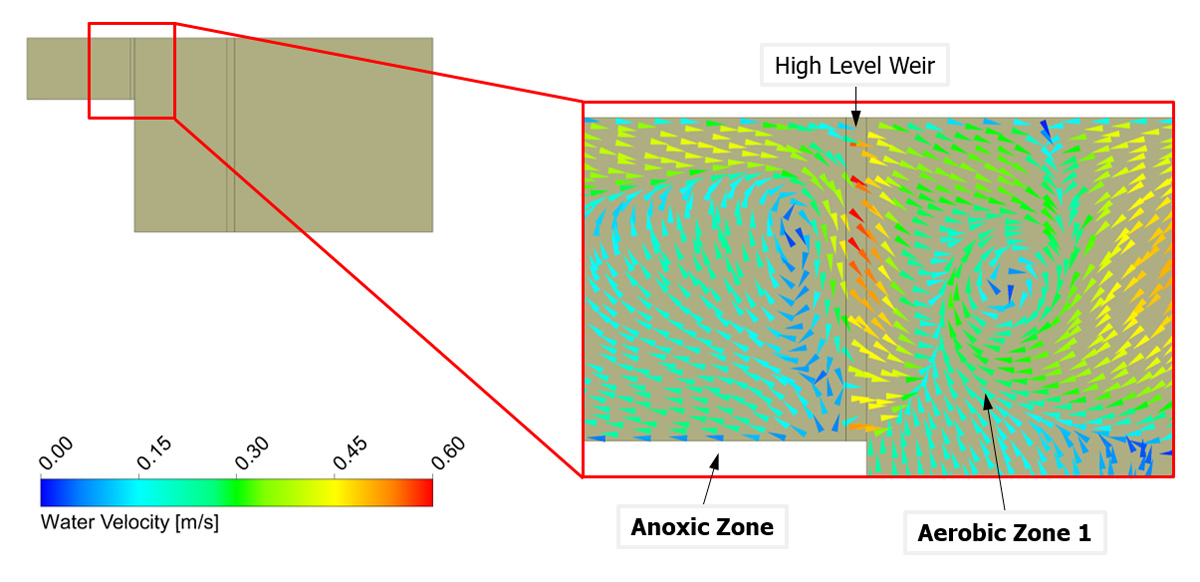
Figure 6: Velocity vectors at the water surface over the high level weir from the anoxic to the aerobic zones at maximum flow – Courtesy MMI Engineering
Final settlement tanks
The final settlement tanks comprise an energy dissipating inlet (EDI) and simplex sludge removal system for extracting the return activated sludge (RAS). In order to characterise the tank performance, a number of state points were assessed to generate a response curve. These state points considered changes to the stirred specific volume index (SSVI), treatment flow and RAS flow.
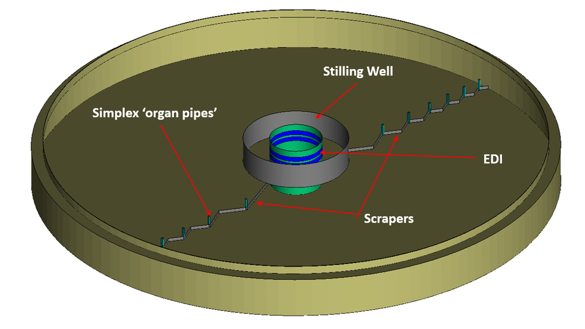
Figure 7: Layout of the FSTs – Courtesy of MMI Engineering
The response curve is presented in Figure 8, presenting the position of the sludge bed against the tank hydraulic loading, the latter being one of the 1D mass flux criterion. In this curve, the ‘0m’ position on the vertical axis represents the bed position relative to the effluent and the point at which the blanket is spilt. The response curve is overlaid on three regions marked in red, amber and green, with red denoting a condition at which the blanket is close to being spilt and inferred to as a failure condition, amber approaching failure and green safe operation.
The response curve shows that over the state points considered, the tank performs well and under steady state conditions, is not close to spilling the sludge blanket up to the recommended hydraulic loading of 80%. Figure 8 presents the distribution of sludge at the hydraulic loading of 80%. The option of including a Stamford baffle was considered but not shown to be of any significant benefit.
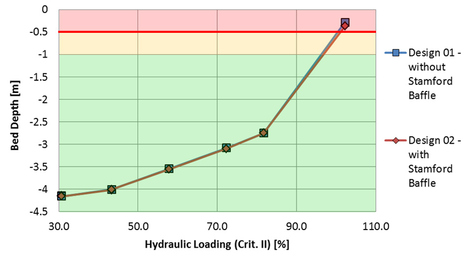
Figure 8. Response curve of the sludge bed position to hydraulic loading – Courtesy of MMI Engineering
Summary
The assessment of the mixing chamber showed that for the Deephams works, in order to achieve best mixing, mixers have to be utilised and positioned at an appropriate location in the system. The use of computational fluid dynamics allowed the positioning of the mixers to be selected for optimum process performance.
The assessment of the aeration lanes found that the weir did not introduce DO back in to the anoxic zone and that there was uniform distribution of both flow and solids load across the width of the aeration lanes. The assessment therefore provided a basis and justification for the design.
Assessment of the FSTs found that the Stamford baffle did not significantly influence the tank performance, and therefore the assessment provided a significant cost saving in the construction of the FSTs.
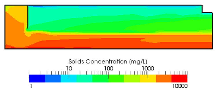
Figure 9. Distribution of sludge at a hydraulic loading of 80% showing good settlement of the sludge – Courtesy of MMI Engineering